Posted 2024-09-16Updated 2024-11-17Missing Semester19 minutes read (About 2833 words)0 visits

Missing Semester Lecture 7 - Debugging and Profiling

MIT The Missing semester Lecture of Your CS Education Lecture 7 - Debugging and Profiling

Profiling

Even if your code functionally behaves as you would expect, that might not be good enough if it takes all your CPU or memory in the process. Algorithms classes often teach big O notation but not how to find hot spots in your programs. Since premature optimization is the root of all evil, you should learn about profilers and monitoring tools. They will help you understand which parts of your program are taking most of the time and/or resources so you can focus on optimizing those parts.

Timing

Similarly to the debugging case, in many scenarios it can be enough to just print the time it took your code between two points. Here is an example in Python using the time module.

import time, random
n = random.randint(1, 10) * 100

# Get current time
start = time.time()

# Do some work
print("Sleeping for {} ms".format(n))
time.sleep(n/1000)

# Compute time between start and now
print(time.time() - start)

# Output
# Sleeping for 500 ms
# 0.5713930130004883

However, wall clock time can be misleading since your computer might be running other processes at the same time or waiting for events to happen. It is common for tools to make a distinction between Real, User and Sys time. In general, User + Sys tells you how much time your process actually spent in the CPU (more detailed explanation here).

Real - Wall clock elapsed time from start to finish of the program, including the time taken by other processes and time taken while blocked (e.g. waiting for I/O or network)
User - Amount of time spent in the CPU running user code
Sys - Amount of time spent in the CPU running kernel code

For example, try running a command that performs an HTTP request and prefixing it with time. Under a slow connection you might get an output like the one below. Here it took over 2 seconds for the request to complete but the process only took 15ms of CPU user time and 12ms of kernel CPU time.

$ time curl https://missing.csail.mit.edu &> /dev/null
real    0m2.561s
user    0m0.015s
sys     0m0.012s

Profilers

CPU

Most of the time when people refer to profilers they actually mean CPU profilers, which are the most common. There are two main types of CPU profilers: tracing and sampling profilers. Tracing profilers keep a record of every function call your program makes whereas sampling profilers probe your program periodically (commonly every millisecond) and record the program’s stack. They use these records to present aggregate statistics of what your program spent the most time doing. Here is a good intro article if you want more detail on this topic.

Most programming languages have some sort of command line profiler that you can use to analyze your code. They often integrate with full fledged IDEs but for this lecture we are going to focus on the command line tools themselves.

In Python we can use the cProfile module to profile time per function call. Here is a simple example that implements a rudimentary grep in Python:

#!/usr/bin/env python

import sys, re

def grep(pattern, file):
    with open(file, 'r') as f:
        print(file)
        for i, line in enumerate(f.readlines()):
            pattern = re.compile(pattern)
            match = pattern.search(line)
            if match is not None:
                print("{}: {}".format(i, line), end="")

if __name__ == '__main__':
    times = int(sys.argv[1])
    pattern = sys.argv[2]
    for i in range(times):
        for file in sys.argv[3:]:
            grep(pattern, file)

We can profile this code using the following command. Analyzing the output we can see that IO is taking most of the time and that compiling the regex takes a fair amount of time as well. Since the regex only needs to be compiled once, we can factor it out of the for.

$ python -m cProfile -s tottime grep.py 1000 '^(import|\s*def)[^,]*$' *.py

[omitted program output]

 ncalls  tottime  percall  cumtime  percall filename:lineno(function)
     8000    0.266    0.000    0.292    0.000 {built-in method io.open}
     8000    0.153    0.000    0.894    0.000 grep.py:5(grep)
    17000    0.101    0.000    0.101    0.000 {built-in method builtins.print}
     8000    0.100    0.000    0.129    0.000 {method 'readlines' of '_io._IOBase' objects}
    93000    0.097    0.000    0.111    0.000 re.py:286(_compile)
    93000    0.069    0.000    0.069    0.000 {method 'search' of '_sre.SRE_Pattern' objects}
    93000    0.030    0.000    0.141    0.000 re.py:231(compile)
    17000    0.019    0.000    0.029    0.000 codecs.py:318(decode)
        1    0.017    0.017    0.911    0.911 grep.py:3(<module>)

[omitted lines]

A caveat of Python’s cProfile profiler (and many profilers for that matter) is that they display time per function call. That can become unintuitive really fast, especially if you are using third party libraries in your code since internal function calls are also accounted for. A more intuitive way of displaying profiling information is to include the time taken per line of code, which is what line profilers do.

For instance, the following piece of Python code performs a request to the class website and parses the response to get all URLs in the page:

#!/usr/bin/env python
import requests
from bs4 import BeautifulSoup

# This is a decorator that tells line_profiler
# that we want to analyze this function
@profile
def get_urls():
    response = requests.get('https://missing.csail.mit.edu')
    s = BeautifulSoup(response.content, 'lxml')
    urls = []
    for url in s.find_all('a'):
        urls.append(url['href'])

if __name__ == '__main__':
    get_urls()

If we used Python’s cProfile profiler we’d get over 2500 lines of output, and even with sorting it’d be hard to understand where the time is being spent. A quick run with line_profiler shows the time taken per line:

$ kernprof -l -v a.py
Wrote profile results to urls.py.lprof
Timer unit: 1e-06 s

Total time: 0.636188 s
File: a.py
Function: get_urls at line 5

Line #  Hits         Time  Per Hit   % Time  Line Contents
==============================================================
 5                                           @profile
 6                                           def get_urls():
 7         1     613909.0 613909.0     96.5      response = requests.get('https://missing.csail.mit.edu')
 8         1      21559.0  21559.0      3.4      s = BeautifulSoup(response.content, 'lxml')
 9         1          2.0      2.0      0.0      urls = []
10        25        685.0     27.4      0.1      for url in s.find_all('a'):
11        24         33.0      1.4      0.0          urls.append(url['href'])

Memory

In languages like C or C++ memory leaks can cause your program to never release memory that it doesn’t need anymore. To help in the process of memory debugging you can use tools like Valgrind that will help you identify memory leaks.

In garbage collected languages like Python it is still useful to use a memory profiler because as long as you have pointers to objects in memory they won’t be garbage collected. Here’s an example program and its associated output when running it with memory-profiler (note the decorator like in line-profiler).

@profile
def my_func():
    a = [1] * (10 ** 6)
    b = [2] * (2 * 10 ** 7)
    del b
    return a

if __name__ == '__main__':
    my_func()

$ python -m memory_profiler example.py
Line #    Mem usage  Increment   Line Contents
==============================================
     3                           @profile
     4      5.97 MB    0.00 MB   def my_func():
     5     13.61 MB    7.64 MB       a = [1] * (10 ** 6)
     6    166.20 MB  152.59 MB       b = [2] * (2 * 10 ** 7)
     7     13.61 MB -152.59 MB       del b
     8     13.61 MB    0.00 MB       return a

Event Profiling

As it was the case for strace for debugging, you might want to ignore the specifics of the code that you are running and treat it like a black box when profiling. The perf command abstracts CPU differences away and does not report time or memory, but instead it reports system events related to your programs. For example, perf can easily report poor cache locality, high amounts of page faults or livelocks. Here is an overview of the command:

perf list - List the events that can be traced with perf
perf stat COMMAND ARG1 ARG2 - Gets counts of different events related to a process or command
perf record COMMAND ARG1 ARG2 - Records the run of a command and saves the statistical data into a file called perf.data
perf report - Formats and prints the data collected in perf.data

Resource Monitoring

Sometimes, the first step towards analyzing the performance of your program is to understand what its actual resource consumption is. Programs often run slowly when they are resource constrained, e.g. without enough memory or on a slow network connection. There are a myriad of command line tools for probing and displaying different system resources like CPU usage, memory usage, network, disk usage and so on.

General Monitoring - Probably the most popular is htop, which is an improved version of top. htop presents various statistics for the currently running processes on the system. htop has a myriad of options and keybinds, some useful ones are: <F6> to sort processes, t to show tree hierarchy and h to toggle threads. See also glances for similar implementation with a great UI. For getting aggregate measures across all processes, dstat is another nifty tool that computes real-time resource metrics for lots of different subsystems like I/O, networking, CPU utilization, context switches, &c.
I/O operations - iotop displays live I/O usage information and is handy to check if a process is doing heavy I/O disk operations
Disk Usage - df displays metrics per partitions and du displays disk usage per file for the current directory. In these tools the -h flag tells the program to print with human readable format. A more interactive version of du is ncdu which lets you navigate folders and delete files and folders as you navigate.
Memory Usage - free displays the total amount of free and used memory in the system. Memory is also displayed in tools like htop.
Open Files - lsof lists file information about files opened by processes. It can be quite useful for checking which process has opened a specific file.
Network Connections and Config - ss lets you monitor incoming and outgoing network packets statistics as well as interface statistics. A common use case of ss is figuring out what process is using a given port in a machine. For displaying routing, network devices and interfaces you can use ip. Note that netstat and ifconfig have been deprecated in favor of the former tools respectively.
Network Usage - nethogs and iftop are good interactive CLI tools for monitoring network usage.

Exercises

Debugging

Use journalctl on Linux or log show on macOS to get the super user accesses and commands in the last day. If there aren’t any you can execute some harmless commands such as sudo ls and check again.

1	$ journalctl --since="1d ago" \| grep sudo

Profiling

Here are some sorting algorithm implementations. Use cProfile and line_profiler to compare the runtime of insertion sort and quicksort. What is the bottleneck of each algorithm? Use then memory_profiler to check the memory consumption, why is insertion sort better? Check now the inplace version of quicksort. Challenge: Use perf to look at the cycle counts and cache hits and misses of each algorithm.

$ python -m cProfile -s tottime sorts.py 1000
         399313 function calls (333375 primitive calls) in 0.214 seconds

   Ordered by: internal time

   ncalls  tottime  percall  cumtime  percall filename:lineno(function)
33794/1000    0.030    0.000    0.031    0.000 sorts.py:23(quicksort)
34144/1000    0.029    0.000    0.034    0.000 sorts.py:32(quicksort_inplace)
     1000    0.025    0.000    0.025    0.000 sorts.py:11(insertionsort)

Using cProfile, it looks like the speed is sorted by: quicksort < quicksort_inplace < insertionsort.

$ kernprof -l -v sorts.py

Wrote profile results to sorts.py.lprof
Timer unit: 1e-06 s

Total time: 0.139251 s
File: sorts.py
Function: insertionsort at line 11

Line #      Hits         Time  Per Hit   % Time  Line Contents
==============================================================
    11                                           @profile
    12                                           def insertionsort(array):
    13
    14     26199       4297.7      0.2      3.1      for i in range(len(array)):
    15     25199       3503.2      0.1      2.5          j = i-1
    16     25199       3986.5      0.2      2.9          v = array[i]
    17    232352      49906.4      0.2     35.8          while j >= 0 and v < array[j]:
    18    207153      41056.8      0.2     29.5              array[j+1] = array[j]
    19    207153      31842.4      0.2     22.9              j -= 1
    20     25199       4511.0      0.2      3.2          array[j+1] = v
    21      1000        147.2      0.1      0.1      return array

Total time: 0.0743435 s
File: sorts.py
Function: quicksort at line 24

Line #      Hits         Time  Per Hit   % Time  Line Contents
==============================================================
    24                                           @profile
    25                                           def quicksort(array):
    26     33346       9455.2      0.3     12.7      if len(array) <= 1:
    27     17173       2242.4      0.1      3.0          return array
    28     16173       3034.6      0.2      4.1      pivot = array[0]
    29     16173      22446.7      1.4     30.2      left = [i for i in array[1:] if i < pivot]
    30     16173      20733.2      1.3     27.9      right = [i for i in array[1:] if i >= pivot]
    31     16173      16431.4      1.0     22.1      return quicksort(left) + [pivot] + quicksort(right)

Using line_profile, we can find that the while loop is the bottleneck of insertion sort, while the double for loops is the bottleneck of quick sort.

Using memory_profiler for insertion sort:

$ python3 -m memory_profiler sorts.py
Filename: sorts.py

Line #    Mem usage    Increment  Occurrences   Line Contents
=============================================================
    11   15.730 MiB   15.730 MiB        1000   @profile
    12                                         def insertionsort(array):
    13
    14   15.730 MiB    0.000 MiB       26096       for i in range(len(array)):
    15   15.730 MiB    0.000 MiB       25096           j = i-1
    16   15.730 MiB    0.000 MiB       25096           v = array[i]
    17   15.730 MiB    0.000 MiB      230871           while j >= 0 and v < array[j]:
    18   15.730 MiB    0.000 MiB      205775               array[j+1] = array[j]
    19   15.730 MiB    0.000 MiB      205775               j -= 1
    20   15.730 MiB    0.000 MiB       25096           array[j+1] = v
    21   15.730 MiB    0.000 MiB        1000       return array

Using memory_profiler for quick sort:

$ python3 -m memory_profiler sorts.py
Filename: sorts.py

Line #    Mem usage    Increment  Occurrences   Line Contents
=============================================================
    24   15.730 MiB   15.730 MiB       33910   @profile
    25                                         def quicksort(array):
    26   15.730 MiB    0.000 MiB       33910       if len(array) <= 1:
    27   15.730 MiB    0.000 MiB       17455           return array
    28   15.730 MiB    0.000 MiB       16455       pivot = array[0]
    29   15.730 MiB    0.000 MiB      157526       left = [i for i in array[1:] if i < pivot]
    30   15.730 MiB    0.000 MiB      157526       right = [i for i in array[1:] if i >= pivot]
    31   15.730 MiB    0.000 MiB       16455       return quicksort(left) + [pivot] + quicksort(right)

The reason why insertion sort is better than quick sort is that in the last step of quick sort, it concatenates which requires extra memory unlike insertion sort which changes its values in place.~~(Although we can’t get this conclusion through my probe result ^^)~~

Using perf to probe:

1
2
3

$ perf record -e cache-misses python3 sorts.py
$ perf record -e cache-references python3 sorts.py
$ perf record -e cycles python3 sorts.py

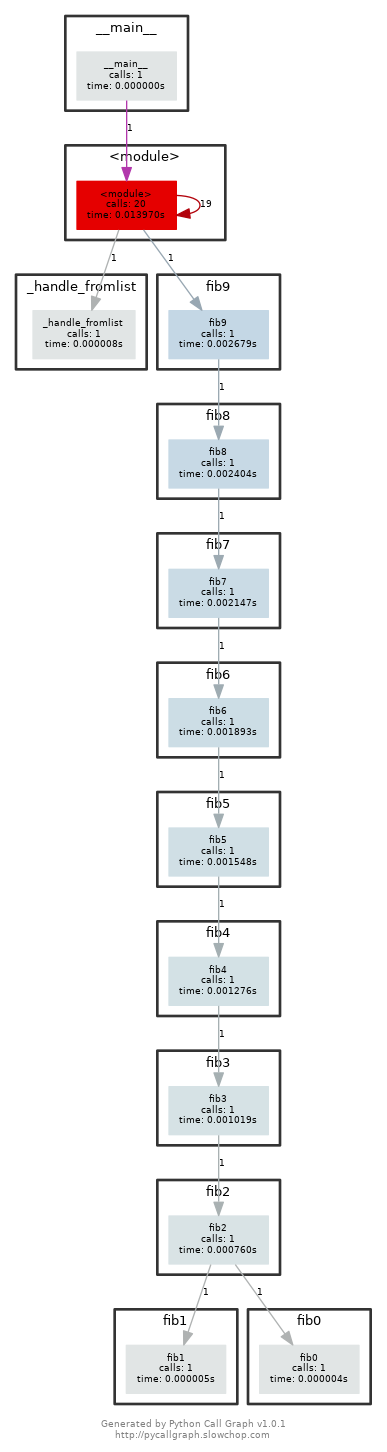
Here’s some (arguably convoluted) Python code for computing Fibonacci numbers using a function for each number.

#!/usr/bin/env python
def fib0(): return 0

def fib1(): return 1

s = """def fib{}(): return fib{}() + fib{}()"""

if __name__ == '__main__':

    for n in range(2, 10):
        exec(s.format(n, n-1, n-2))
    # from functools import lru_cache
    # for n in range(10):
    #     exec("fib{} = lru_cache(1)(fib{})".format(n, n))
    print(eval("fib9()"))

Put the code into a file and make it executable. Install prerequisites: pycallgraph and graphviz. (If you can run dot, you already have GraphViz.) Run the code as is with pycallgraph graphviz -- ./fib.py and check the pycallgraph.png file. How many times is fib0 called?. We can do better than that by memoizing the functions. Uncomment the commented lines and regenerate the images. How many times are we calling each fibN function now?

After execute pycall graph graphviz -- ./fib.py, the generated pycallgraph.png file is:

We can find that the fib0 is called 21 times.

After we uncomment the commented lines and regenerate the images, we can find the graph looks like this:
re_pycallgraph

A common issue is that a port you want to listen on is already taken by another process. Let’s learn how to discover that process pid. First execute python -m http.server 4444 to start a minimal web server listening on port 4444. On a separate terminal run lsof | grep LISTEN to print all listening processes and ports. Find that process pid and terminate it by running kill <PID>.

execute python -m http.server 4444 to start a web server:

1 2	$ python3 -m http.server 4444 Serving HTTP on 0.0.0.0 port 4444 (http://0.0.0.0:4444/) ...

run lsof | grep LISTEN:

1 2	$ lsof \| grep LISTEN python3 8525 root 3u IPv4 31943 0t0 TCP *:krb524 (LISTEN)

kill server:

$ kill 8525

$ python3 -m http.server 4444
Serving HTTP on 0.0.0.0 port 4444 (http://0.0.0.0:4444/) ...
已终止

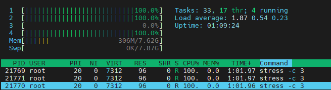
Limiting a process’s resources can be another handy tool in your toolbox. Try running stress -c 3 and visualize the CPU consumption with htop. Now, execute taskset --cpu-list 0,2 stress -c 3 and visualize it. Is stress taking three CPUs? Why not? Read man taskset.

Run stress -c 3:

1 2	$ stress -c 3 stress: info: [21768] dispatching hogs: 3 cpu, 0 io, 0 vm, 0 hdd

Then run htop we can find:
Execute taskset --cpu-list 0,2 stress -c 3 and run htop: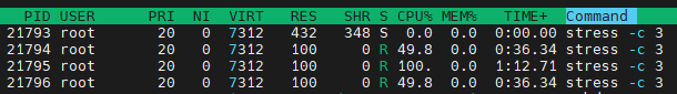

We can find stress just take one cpu. Because in man taskset said: The Linux scheduler will honor the given CPU affinity and the process will not run on any other CPUs.

Missing Semester Lecture 7 - Debugging and Profiling

Profiling

Timing

Profilers

CPU

Memory

Event Profiling

Resource Monitoring

Exercises

Debugging

Profiling

Comments

Categories

Recents

Archives

Tags